Chapter 1: Using Excel Worksheets and Workbooks

This chapter covers: Understanding what Excel is used for, looking at what’s new in Excel 2013, learning the parts of an Excel window, Navigating Excel worksheets, and Introducing Excel’s Ribbon.

 1.1. Identifying What Excel Is Good For

Excel, as you probably know, is the world’s most widely used spreadsheet software and part of the Microsoft Office suite. 

Excel’s specialty, is performing numerical calculations, but Excel is also very useful for non-numeric applications. Here are just a few of the uses for Excel: 

• Number crunching: Create budgets, tabulate expenses, analyze survey results, and perform just about any type of financial analysis you can think of.
• Creating charts: Create a wide variety of highly customizable charts.
• Organizing lists: Use the row-and-column layout to store lists efficiently.
• Text manipulation: Clean up and standardize text-based data.
• Accessing other data: Import data from a wide variety of sources.
• Creating graphics and diagrams: Use Shapes and SmartArt to create professional looking diagrams.
• Automating complex tasks: Perform a tedious task with a single mouse click with Excel’s macro capabilities.

1.2. Seeing what’s New in Excel 2013

When a new version of Microsoft Office is released, sometimes Excel gets lots of new features and other times it gets very few new features. In the case of Office 2013, Excel got quite a few new features. Here’s a quick summary of what’s new in Excel 2013, relative to Excel 2010:

• Support for other devices: Excel is available for other devices, including touch sensitive devices such as Windows RT tablets and Windows phones.
• New aesthetics: Excel has a new “flat” look and displays an (optional) graphic in the title bar. The default color scheme is white, but you can choose from two other color schemes (light gray and dark gray) in the General tab of the Excel Options dialog box.
• Single document interface: Excel no longer supports the option to display multiple workbooks in a single window. Each workbook has its own top-level Excel window and Ribbon.
• Enhanced chart formatting: Modifying charts is significantly easier.
• New worksheet functions: Excel 2013 supports dozens of new worksheet functions.
• Backstage: The Backstage screen has been reorganized and is easier to use.

NB: A version is an updated software with additional features or functionalities. For Microsoft Office software, there have been a lot of versions: examples: 

• MS Office xp
• MS Office 2000
• MS Office 2003
• MS Office 2007 
• MS Office 2010
• MS Office 2013, the one that will are using for Excel and Powerpoint
• MS Office 2016

1.3. Understanding Workbooks and Worksheets

The work you do in Excel is performed in a workbook file. You can have as many workbooks open as you need, and each one appears in its own window. By default, Excel workbooks use an .xlsx file extension.

Each workbook contains one or more worksheets, and each worksheet is made up of individual cells. Each cell can contain a value, a formula, or text. 

To understand important pieces of Excel and what each of them does, click here  Understanding Excel Working Environment.

1.4. Moving around a Worksheet

Every worksheet consists of rows (numbered 1 through 1,048,576) and columns (labeled A through XFD). Column labeling works like this: After column Z comes column AA, which is followed by AB, AC, and so on. After column AZ comes BA, BB, and so on. After column ZZ is AAA, AAB, and so on. 

The intersection of a row and a column is a single cell, and each cell has a unique address made up of its column letter and row number. For example, the address of the upper-left cell is A1. The address of the cell at the lower right of a worksheet is XFD1048576.

This means that the first column is lettered A and the last column is lettered XFD. The first row is numbered 1 and the last row is numbered 1048576.

To display the hidden part of a worksheet, you use scroll buttons (horizontal and vertical).

Navigating with your keyboard

You can use the standard navigational keys on your keyboard to move around a worksheet. These keys work just as you’d expect: The down arrow moves the active cell down one row, the right arrow moves it one column to the right, and so on. Page Up and Page Down move the active cell up or down one full window. 

Navigating with your mouse

 To change the active cell by using the mouse, just click another cell, and it becomes the active cell. If the cell that you want to activate isn’t visible in the workbook window, you can use the scroll bars to scroll the window in any direction. 

1.5. Introducing Excel’s Ribbon Tabs

Traditional menus and toolbars were replaced with the Ribbon in Excel 2013. A ribbon is a collection of icons at the top of the screen. The words above the icons are known as tabs: the Home tab, the Insert tab, and so on. Most users find that the Ribbon is easier to use than the old menu system; it can also be customized to make it even easier to use.

The Ribbon looks like the following: 

(NB: tabs groups, icons, etc. they all make a ribbon). The HOME tab is the one that is selected for this ribbon! If another tab was selected, then the appearance would change (icons, etc.)

• Tabs are HOME, INSERT, PAGE LAYOUT, FORMULAS, DATA, REVIEW, VIEW, DEVELOPER, ADD-INS. 
• Each Tab has groups. Example HOME tab has groups like Clipboard, Font, Alignment, Number, Styles, Cells, and Editing.
• Each group has icons. Example Font group has icons like B, I, U, and so on.

To read more about ribbons in Excel click here Understanding Excel Ribbon tabs.

1.6. Creating Your First Excel Workbook

Start Excel and make sure that you have an empty workbook displayed by selecting Blank workbook from the Start screen.

To create a new, blank workbook when Excel is already open, press Ctrl+N (the shortcut key for File ➪ New ➪ Blank Workbook).

The sales projection will consist of two columns of information. Column A will contain the month names, and column B will store the projected sales numbers. You start by entering some descriptive titles into the worksheet. Here’s how to begin:

1. Move the cell pointer to cell A1 (the upper-left cell in the worksheet) if needed by using the navigation (arrow) keys. The Name box displays the cell’s address.
2. Type Month into cell A1 and press Enter. Depending on your setup, either Excel moves the cell pointer to a different cell or the pointer remains in cell A1.
3. Move the cell pointer to B1, type Projected Sales, and press Enter. The text extends beyond the cell width, but don’t worry about that for now.

Filling in the month names

In this step, you enter the month names in column A.

1. Move the cell pointer to A2 and type Jan (an abbreviation for January). At this point, you can enter the other month name abbreviations manually or you can let Excel do some of the work by taking advantage of the AutoFill feature.
2. Make sure that cell A2 is selected. Notice that the active cell is displayed with a heavy outline. At the bottom-right corner of the outline, you’ll see a small square known as the fill handle. Move your mouse pointer over the fill handle, click, and drag down until you’ve highlighted from cell A2 down to cell A13.
3. Release the mouse button, and Excel automatically fills in the month names.

Entering the sales data

Next, you provide the sales projection numbers in column B. Assume that January’s sales are projected to be $50,000, and that sales will increase by 3.5 percent in each subsequent month.

1. Move the cell pointer to B2 and type 50000, the projected sales for January. You could type a dollar sign and comma to make the number more legible, but we will do the number formatting a bit later.

To enter a formula to calculate the projected sales for February, move to cell B3 and type the following: =B2*103.5%  , when you press Enter, the cell displays 51750. The formula returns the contents of cell B2, multiplied by 103.5%. In other words, February sales are projected to be 103.5% of the January sales — a 3.5% increase.

3. The projected sales for subsequent months use a similar formula, but rather than retype the formula for each cell in column B, take advantage of the Auto Fill feature. Make sure that cell B3 is selected. Click the cell’s fill handle, drag down to cell B13, and release the mouse button.

Summing the values

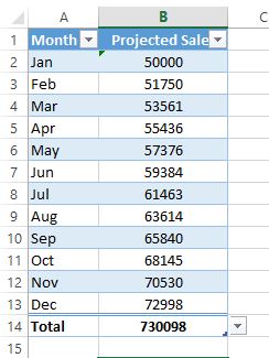
 The worksheet displays the monthly projected sales, but what about the total projected sales for the year? Because this range is a table, it’s simple:

1. Activate any cell in the table.
2. Choose Table Tool from Insert Tab, Tables Group➪ Ok➪Design Tab ➪ Table Style Options Group ➪ Total Row. Excel automatically adds a new row to the bottom of your table, including a formula that calculates the total of the Projected Sales column.
3. If you’d prefer to see a different summary formula (for example, average), click cell B14 and choose a different summary formula from the drop-down list.

If you have followed all the given steps, you should get something like the following:

Saving your workbook

Until now, everything that you’ve done has occurred in your computer’s memory. If the power should fail, all may be lost — unless Excel’s AutoRecover feature happened to kick in. It’s time to save your work to a file on your hard drive. 

1. Click the Save button on the Quick Access Toolbar. (This button looks like an old-fashioned floppy disk, popular in the previous century.) Because the workbook hasn’t been saved yet and still has its default name, Excel responds with a backstage screen that lets you choose the location for the workbook file. The Backstage screen lets you save the file to an online location or to your local computer.
2. Select Computer, and then click Browse. Excel displays the Save As dialog box.

In the File name text box, enter a name (such as Monthly Sales Projection), and then click Save or press Enter. Excel saves the workbook as a file. The workbook remains open so that you can work with it some more.